Does the price of a sealed Lego® set automatically rise when production ends? Many collectors and investors plan around that assumption. The short answer is: no, retirement does not make it automatic.
There is a clear pattern in Brickfact's market data. Twelve months after the recorded retirement month, the median estimated market value was 22.3% higher. After 24 months, it was 41.0% higher. At the same time, almost one in five sets still had no positive change after a year. The median for sets retired in 2022 was actually negative at that point.
That distinction matters. Retirement can reduce supply, but it cannot create demand, secure a good purchase price or guarantee a buyer when you want to sell.
The first three years in four numbers
- After 3 months: median market-value change of +6.9%; 26.5% of sets were no higher than in their retirement month.
- After 12 months: median +22.3%; 18.8% had no positive change.
- After 24 months: median +41.0%; 13.5% had no positive change.
- After 36 months: median +55.5%; 10.9% had no positive change.
The median changes refer to Brickfact's market-value estimate for sealed sets; the other percentages show the share of sets with no positive change. They are not sale proceeds or returns on your own purchase price.
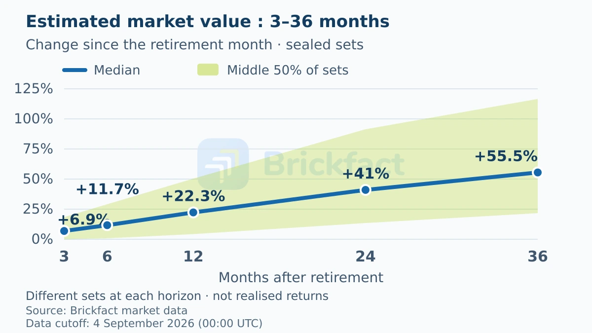
How Lego® market values developed after retirement
The 25th and 75th percentiles show the middle half of the cumulative changes, making the wide differences between individual sets visible. Alongside the total median change, the table shows annualized estimated value growth (CAGR): the median equivalent compounded rate per year. The charts continue to show cumulative changes.
| Time after retirement month | Sets | 25th percentile | Median total change | Median annualized change (CAGR) | 75th percentile | No positive change |
|---|---|---|---|---|---|---|
| 3 months | 3,101 | 0.0% | +6.9% | – | +18.4% | 26.5% |
| 6 months | 3,149 | +0.8% | +11.7% | – | +29.1% | 23.4% |
| 12 months | 3,117 | +4.3% | +22.3% | +22.3% | +50.4% | 18.8% |
| 24 months | 2,836 | +13.5% | +41.0% | +18.8% | +91.4% | 13.5% |
| 36 months | 2,565 | +21.7% | +55.5% | +15.9% | +116.6% | 10.9% |
| 48 months | 2,218 | +34.4% | +75.9% | +15.2% | +146.5% | 6.9% |
| 60 months | 1,882 | +47.3% | +96.9% | +14.5% | +175.6% | 4.9% |
| 84 months | 1,509 | +67.0% | +124.7% | +12.3% | +222.8% | 2.3% |
| 120 months | 695 | +79.4% | +157.1% | +9.9% | +286.7% | 2.3% |
For each set, we calculate (comparison-month value / retirement-month value)^(12 / months) − 1, then take the median and express it as a percentage rounded to one decimal place. We use the unrounded monthly estimates, not the rounded cumulative medians. A dash means no annualized figure is shown for periods shorter than a year. CAGR is not growth observed every year or a realized investment return; purchase prices, fees, storage costs and inflation are not accounted for. Annualizing also does not make the samples identical across horizons.
Here is how to read one row: among sets with sufficient data after 24 months, the middle half ranged from +13.5% to +91.4%. The +41.0% median is therefore not a standard result you can expect from any set you choose. The spread is large.
The sample size also changes between horizons. We only included a set at each point if it had enough observations in both its retirement month and the relevant comparison month. Longer comparisons also require an earlier retirement date: the ten-year result cannot include a set that retired only five years ago.
What happened after four, five, seven and ten years?
The pattern did not end at three years. After 48 months, the median estimated market value was 75.9% above the retirement-month baseline, across 2,218 sets. After 60 months, the median was +96.9%, based on 1,882 sets. These are cumulative changes over four and five years, not annual rates and not money received from selling a collection.
The five-year spread is more informative than the median alone. The middle half ranged from +47.3% to +175.6%. A set near the lower quartile therefore had a very different estimated-value history from one near the upper quartile, even though both belonged to the same horizon. Meanwhile, 4.9% had no positive change at all. A longer holding period did not turn every observed set into a winner.
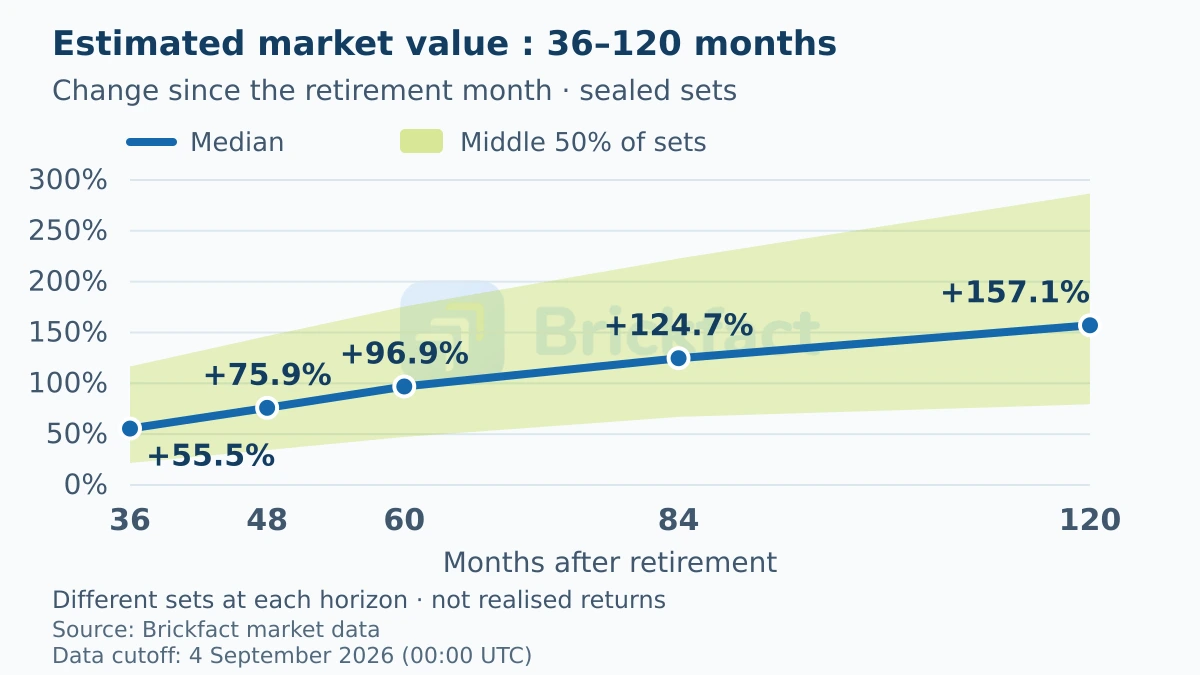
At 84 months, the median was +124.7% across 1,509 sets. At 120 months, it reached +157.1%, but the qualifying group had narrowed to 695 sets. Those ten-year observations concern sets retired between 2011 and 2016. They do not describe the future of sets retiring today, and the lower sample count is not a count of sets that lost value or disappeared from the market.
The ten-year middle half ranged from +79.4% to +286.7%. Looking further into the distribution, the 10th and 90th percentiles were +35.9% and +466.3%. Those percentiles are neither minimum and maximum outcomes nor a confidence interval for the median. They describe the spread across the qualifying sets. The very wide range is a reason to be cautious about using a single long-term percentage as a buying rule.
What changes when we track the same 622 sets?
The main table answers a separate question at each horizon: what happened to every set with enough data for that particular comparison? Its rows do not follow one unchanged collection. Comparing their medians mixes elapsed time with changes in the sets included.
To examine that distinction, we also selected 622 sets with qualifying observations at every one of the nine tested horizons, as well as the retirement-month baseline. The table below shows selected horizons for that fixed group. Its membership stays the same from row to row. Both medians use this fixed group; annualized changes are calculated from each set’s retirement-month baseline, not between successive table rows.
| Time after retirement month | Same sets | Median total change | Median annualized change (CAGR) | No positive change |
|---|---|---|---|---|
| 12 months | 622 | +39.1% | +39.1% | 17.2% |
| 36 months | 622 | +86.0% | +23.0% | 5.6% |
| 60 months | 622 | +113.5% | +16.4% | 3.4% |
| 84 months | 622 | +131.4% | +12.7% | 2.4% |
| 120 months | 622 | +150.0% | +9.6% | 2.4% |
The difference is already visible after a year. The fixed group's median was +39.1%, compared with +22.3% in the larger twelve-month sample. That is not a contradiction: the older sets with a complete observation history were a different group. At ten years, the fixed-group median was +150.0%, compared with +157.1% for all 695 sets qualifying for that single horizon.
Keeping membership constant removes one source of ambiguity, but it does not make the group representative of every retired set. It still favours older sets with sufficiently complete price histories. Nor does it control for changing demand, remakes or the wider market. The observations show higher cumulative medians at later sampled horizons within the same group; they do not establish what caused that pattern or show that every set rose continuously between those points.
Why a longer holding period needs a different calculation
The long-term figures make storage, condition and the timing of a sale more relevant to a practical decision. Keeping a box sealed for a decade requires space and protection from damage. Those costs are not subtracted from the estimates, and the study does not measure how quickly a buyer could have been found at the recorded value.
Inflation also matters: the reported market-value changes are based on nominal euro values, not changes in purchasing power. Comparing the result with a savings account, shares or another use of your money would require matched dates, cash flows, costs and risks. The study does not make that comparison.
Do not subtract the pooled five-year median from the ten-year median and call the difference a return earned during the intervening years. The groups differ, and a difference between medians is not the median of individual later-period changes. For an actual set, the relevant starting point remains its own purchase price and the net proceeds you could realistically receive.
Retirement does not switch scarcity on overnight
A set is retired when its regular production run ends. The market does not empty overnight. Retailers can still have stock, private sellers can hold unopened boxes and heavily purchased sets may remain widely available.
Positive changes were least widespread at the earliest horizon. After three months, the 25th percentile was exactly zero, and more than a quarter of sets had not moved above their estimated market value in the retirement month.
For you, that means retirement is information about supply, not a complete reason to buy. Before making a decision, you still need to ask:
- How does the current retailer price compare with RRP/MSRP?
- Are there close substitutes or likely remakes?
- Is there an identifiable collector audience beyond a short-lived trend?
- How stable has the set's own price history been?
- What fees, postage and storage costs would a later sale create?
Our analysis does not test those factors separately. It shows why the word “retired” cannot replace them.
The retirement year changed the result substantially
A pooled median combines very different market periods. We therefore also grouped sets by the year in which they retired. The recent cohorts show why a fixed “retirement return” would be misleading.
| Retirement year | Sets at 12 months | Median at 12 months | Sets at 24 months | Median at 24 months |
|---|---|---|---|---|
| 2020 | 162 | +8.4% | 165 | +24.7% |
| 2021 | 374 | +18.2% | 322 | +18.5% |
| 2022 | 299 | −1.8% | 308 | +3.9% |
| 2023 | 283 | +10.8% | 281 | +23.9% |
| 2024 | 226 | +11.7% | – | – |
The 2022 cohort is the clearest counterexample to the claim that every retired set rises quickly. After twelve months, its median was 1.8% below the retirement-month market value, and 55.2% of the sets had no positive change. Even after 24 months, the median was only +3.9%, while 43.2% still were not above their starting point.
This analysis alone cannot tell us why 2022 was weaker. Doing that would require separate tests of demand, retailer inventory, discounts and the mix of products. We use the cohort as a warning, not as a post-hoc explanation.
We deliberately do not show a 24-month figure for 2024. A complete two-year period was not available for that cohort at the study's data cutoff.
Expensive sets were not automatically better
RRP/MSRP was not a simple quality filter either. For sets with a documented euro RRP, we split the 24-month change by documented euro RRP band.
| Euro RRP | Sets | Median after 24 months |
|---|---|---|
| Under €30 | 1,536 | +40.7% |
| €30 to €59.99 | 634 | +46.1% |
| €60 to €119.99 | 464 | +40.8% |
| €120 or more | 176 | +35.7% |
The medians are fairly close, while outcomes within every band vary widely. This does not show that small sets are inherently better or that large sets are worse. Most importantly, the table measures change from the estimated market value in the retirement month. It does not compare your purchase price with a later sale.
A set with a €100 RRP might be available for €70 shortly before retirement while its estimated market value is €85. Purchase price, RRP and market value are three different numbers. A personal return calculation also needs your actual purchase cost and every selling expense.
What this means for collectors
If you want to keep a set anyway, retirement is primarily a timing signal: replacing it may become harder after production ends. The study does not say that you should accept any asking price because of that signal.
Look at the specific set rather than relying on the overall median. Brickfact's Lego® Value Checker shows the estimated value of a sealed set and its price history. The Lego® retirement list helps you find sets expected to retire or already retired. A forecast can move, and retailer inventory can outlast production.
Condition matters as well. This study covers sealed sets. Built sets, damaged boxes, missing minifigures and discoloured pieces belong to a different market and can have very different values.
What this means for Lego® investors
The most useful finding is not the highest percentage; it is the range. After twelve months, the 25th percentile was +4.3% and the 75th percentile was +50.4%. Two sets with the same retirement month could therefore follow very different paths.
A sensible calculation starts before you buy:
- Record the purchase price: RRP/MSRP is not a substitute for what you paid.
- Keep market value separate: an estimated value is not a realised sale.
- Include costs: marketplace and payment fees, packing, postage, storage and damage can reduce the result.
- Consider liquidity: a high estimate is less useful when a set rarely finds a buyer.
- Do not overrate one retirement date: production plans and remaining inventory can change.
This study does not measure realised investment returns. It cannot tell you how much an investor kept after costs. It measures the historical movement of a market-value estimate.
Methodology of the Brickfact retirement study
Data cutoff: 4 September 2026. The analysis uses historical Brickfact market values in euros and the retirement month stored in the Brickfact set catalogue.
We began with 4,416 catalogue records marked as retired with a dated retirement between 2011 and 2024. One record with an impossible lifecycle was excluded, leaving 4,415 sets with a plausible retirement month. Of those, 3,161 had at least ten observed price days in the retirement month. The final sample depends on the comparison point and ranges from 3,149 sets after six months to 695 after 120 months.
The calculation works as follows:
- We first averaged multiple observations for the same set on the same day. A day with several entries therefore did not receive more weight than another observed day.
- For each set, we calculated the median of its observed daily values in the calendar month of retirement.
- We repeated that process 3, 6, 12, 24, 36, 48, 60, 84 and 120 months later.
- A comparison was included only when both calendar months contained at least ten observed price days.
- We calculated the relative change for each set before aggregating the median, percentiles and share with no positive change. Large and small sets receive equal weight.
The source is Brickfact's historical market-price series for sealed sets. We did not use Brickfact user accounts, portfolios or personal transactions.
For the fixed-group comparison, we additionally required each set to pass the same ten-observed-day threshold at all nine horizons. This left 622 sets. The main table retains the broader, horizon-specific samples; the fixed-group table does not replace them. The data cutoff and the original three-to-36-month results remain unchanged in this expanded analysis.
Limitations
- Market value is an estimate of the secondary market, not a guaranteed selling price.
- The stored retirement date is a calendar month rather than an exact day. Retrospective catalogue changes can affect historical assignments.
- Only sets with enough observations in both comparison months qualify. Thinly traded sets may therefore be underrepresented.
- The main table's nine horizon-specific samples are not identical. The ten-year sample contains retirement years 2011–2016; later retirement cohorts cannot yet supply ten-year observations at the cutoff.
- The fixed group keeps membership constant, but requiring complete observations can introduce selection bias. It does not establish causality or eliminate differences between historical market periods.
- Fees, postage, storage, taxes and inflation are not deducted.
- Retailer prices and RRP/MSRP are not matched to later sales. The RRP table only describes documented euro RRP bands.
- The analysis describes an association. It does not prove that retirement alone caused a price change.
Conclusion: The cumulative median rose, but not every set did
The horizon-specific samples show median estimated market-value changes of +22.3% after twelve months, +41.0% after 24 months and +157.1% after ten years. The ten-year result concerns a smaller, older group, not a forecast for the complete catalogue. A separate comparison of the same 622 sets also shows higher cumulative medians at later sampled horizons, with +150.0% at ten years.
The other side is just as important: 18.8% of sets were not above their starting value after a year, and the 2022 retirement cohort had a negative twelve-month median. Retirement is not a promise of returns; it is one input into a wider analysis.
When you assess an individual set, use the overall median only as context. The set's own price history, your purchase price and realistic selling costs determine the result.
Frequently asked questions about Lego® prices after retirement
Does every Lego® set rise in value after retirement?
No. In our sample, 18.8% of sets had no positive market-value change after twelve months and 13.5% had no positive change after 24 months. Individual retirement-year cohorts also performed well below the pooled median.
How quickly do Lego® prices rise after retirement?
The median change was +6.9% after three months, +22.3% after twelve months and +41.0% after 24 months. These are aggregated historical values, not a forecast for a particular set.
Is market value the same as my sale proceeds?
No. Market value is an estimate for a sealed set. Your actual selling price determines gross proceeds; fees, shipping, condition, storage and taxes affect the net result.
Does the study prove that retirement causes prices to rise?
No. The analysis compares the market value in the stored retirement month with market values in later months. It does not causally separate demand, discounts, remaining inventory, remakes or other influences.
When is the best time to buy a retiring set?
This study does not answer that question. Doing so would require a separate analysis of retailer prices and discounts before production ends. A retirement date on its own is not enough to make the decision.